Clebsch–Gordan coefficients
In physics, the Clebsch–Gordan coefficients are sets of numbers that arise in angular momentum coupling under the laws of quantum mechanics.
In more mathematical terms, the CG coefficients are used in representation theory, particularly of compact Lie groups, to perform the explicit direct sum decomposition of the tensor product of two irreducible representations into irreducible representations, in cases where the numbers and types of irreducible components are already known abstractly. The name derives from the German mathematicians Alfred Clebsch (1833–1872) and Paul Gordan (1837–1912), who encountered an equivalent problem in invariant theory.
In terms of classical mathematics, the CG coefficients, or at least those associated to the group SO(3), may be defined much more directly, by means of formulae for the multiplication of spherical harmonics. The addition of spins in quantum-mechanical terms can be read directly from this approach. The formulas below use Dirac's bra-ket notation.
Clebsch–Gordan coefficients
Clebsch–Gordan coefficients are the expansion coefficients of total angular momentum eigenstates in an uncoupled tensor product basis.
Below, this definition is made precise by defining angular momentum operators, angular momentum eigenstates, and tensor products of these states.
From the formal definition of angular momentum, recursion relations for the Clebsch–Gordan coefficients can be found. To find numerical values for the coefficients a phase convention must be adopted. Below the Condon–Shortley phase convention is chosen.
Angular momentum operators
Angular momentum operators are self-adjoint operators  ,
,  , and
, and  that satisfy the commutation relations
![[\textrm{j}_k,\textrm{j}_l] = \textrm{j}_k \textrm{j}_l - \textrm{j}_l \textrm{j}_k = i\hbar \sum_m
\varepsilon_{kl m}\textrm{j}_m, \quad\mathrm{where}\quad k,l,m \in (x,y,z)](/2012-wikipedia_en_all_nopic_01_2012/I/4f3e98154906fc8615c3cb6986c845b7.png)
where  is the Levi-Civita symbol. Together the three operators define a "vector operator":
![\mathbf{j} = [\textrm{j}_x,\textrm{j}_y,\textrm{j}_z]](/2012-wikipedia_en_all_nopic_01_2012/I/2798ffe27b0c73c19106a4bd40dfecd4.png)
By developing this concept further, one can define an operator as an "inner product" of  with itself:
It is an example of a Casimir operator.
We also define raising ( ) and lowering (
 ) operators:
Angular momentum states
It can be shown from the above definitions that  commutes with , and
![[\mathbf{j}^2, \textrm{j}_k] = 0\ \mathrm{for}\ k = x,y,z](/2012-wikipedia_en_all_nopic_01_2012/I/57b360fd13cc63698bc29ae9a7307c88.png)
When two Hermitian operators commute a common set of eigenfunctions exists. Conventionally and are chosen. From the commutation relations the possible eigenvalues can be found. The result is
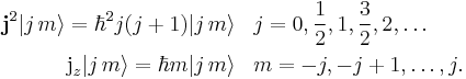
The raising and lowering operators change the value of 
with

A (complex) phase factor could be included in the definition of  The choice made here is in agreement with the Condon and Shortley phase conventions. The angular momentum states must be orthogonal (because their eigenvalues with respect to a Hermitian operator are distinct) and they are assumed to be normalized
Tensor product space
Let  be the
  dimensional vector space spanned by the states

and  the
the  dimensional vector space spanned by

The tensor product of these spaces, 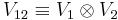 , has a
 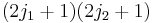 dimensional uncoupled basis

Angular momentum operators acting on  can be defined by

and

Total angular momentum operators are defined by

The total angular momentum operators satisfy the required commutation relations
![[\textrm{J}_k,\textrm{J}_l] = i\hbar\epsilon_{klm}\textrm{J}_m, \quad \mathrm{where}\quad k,l,m \in (x,y,z)](/2012-wikipedia_en_all_nopic_01_2012/I/00d41736fc3ef6b1751fc2c642811491.png)
and hence total angular momentum eigenstates exist
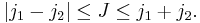
It can be derived that  must satisfy the triangular condition
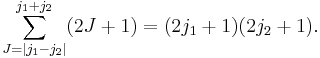
The total number of total angular momentum eigenstates is equal to the dimension of
The total angular momentum states form an orthonormal basis of

Formal definition of Clebsch–Gordan coefficients
The total angular momentum states can be expanded with the use of the completeness relation in the uncoupled basis
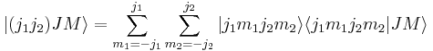
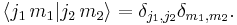
The expansion coefficients  are called Clebsch–Gordan coefficients.
Applying the operator
to both sides of the defining equation shows that the Clebsch–Gordan coefficients can only be nonzero when
Recursion relations
The recursion relations were discovered by the physicist Giulio Racah. Applying the total angular momentum raising and lowering operators
to the left hand side of the defining equation gives

Applying the same operators to the right hand side gives
![\begin{align}
\textrm{J}_\pm & \sum_{m_1m_2} |j_1m_1\rangle|j_2m_2\rangle \langle j_1m_1j_2m_2|JM\rangle\\
& =\sum_{m_1m_2}\left[ C_\pm(j_1,m_1)|j_1 m_1\pm 1\rangle |j_2m_2\rangle
%2BC_\pm(j_2,m_2)|j_1 m_1\rangle |j_2 m_2\pm 1\rangle \right]
\langle j_1 m_1 j_2 m_2|J M\rangle \\
&= \sum_{m_1m_2} |j_1m_1\rangle|j_2m_2\rangle \left[
C_\pm(j_1,m_1\mp 1) \langle j_1 {m_1\mp 1} j_2 m_2|J M\rangle
%2BC_\pm(j_2,m_2\mp 1) \langle j_1 m_1 j_2 {m_2\mp 1}|J M\rangle \right].
\end{align}](/2012-wikipedia_en_all_nopic_01_2012/I/16cb82543b2c3e85eb95f5555f9da492.png)
where
Combining these results gives recursion relations for the Clebsch–Gordan coefficients

Taking the upper sign with  gives
gives

In the Condon and Shortley phase convention the coefficient  is taken real and positive. With the last equation all other Clebsch–Gordan coefficients
  can be found. The normalization is fixed by the requirement that the sum of the squares, which corresponds to the norm of the state
  must be one.
The lower sign in the recursion relation can be used to find all the Clebsch–Gordan coefficients with  . Repeated use of that equation gives all coefficients.
This procedure to find the Clebsch–Gordan coefficients shows that they are all real (in the Condon and Shortley phase convention).
Explicit expression
For an explicit expression of the Clebsch–Gordan coefficients and tables with numerical values, see table of Clebsch–Gordan coefficients.
Orthogonality relations
These are most clearly written down by introducing the alternative notation

The first orthogonality relation is

(using the completeness relation that  )and the second

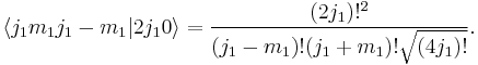
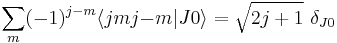
Special cases
For  the Clebsch–Gordan coefficients are given by
For  and we have

For 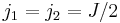 and
and  we have
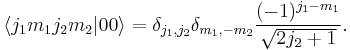
For 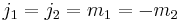 we have
Symmetry properties
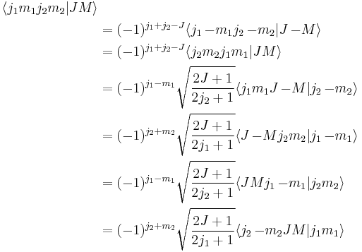
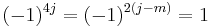
A convenient way to derive these relations is by converting the Clebsch–Gordan coefficients to 3-jm symbols using the equation given below. The symmetry properties of 3-jm symbols are much simpler. Care is needed when simplifying phase factors, because the quantum numbers can be integer or half integer, e.g.,  is equal to 1 for integer
  and equal to −1 for half-integer . The following relations, however, are valid in either case:
and for  ,
,  and appearing in the same Clebsch–Gordan coefficient:

Relation to 3-jm symbols
Clebsch–Gordan coefficients are related to 3-jm symbols which have more convenient symmetry relations.

Relation to Wigner D-matrices

Other Properties
SU(N) Clebsch–Gordan coefficients
For arbitrary groups and their representations, Clebsch–Gordan coefficients are not known in general. However, algorithms to produce Clebsch–Gordan coefficients for the Special unitary group are known.[1] A web interface for tabulating SU(N) Clebsch–Gordan coefficients is readily available.
See also
Further reading
- Biedenharn, L. C.; Louck, J. D. (1981). Angular Momentum in Quantum Physics. Reading, Massachusetts: Addison-Wesley. ISBN 0201135078.
- Brink, D. M.; Satchler, G. R. (1993). "Ch. 2". Angular Momentum (3rd ed.). Oxford: Clarendon Press. ISBN 0-19-851759-9.
- Condon, Edward U.; Shortley, G. H. (1970). "Ch. 3". The Theory of Atomic Spectra. Cambridge: Cambridge University Press. ISBN 0-521-09209-4.
- Edmonds, A. R. (1957). Angular Momentum in Quantum Mechanics. Princeton, New Jersey: Princeton University Press. ISBN 0-691-07912-9.
- Messiah, Albert (1981). "Ch. XIII". Quantum Mechanics (Volume II). New York: North Holland Publishing. ISBN 0-7204-0045-7.
- Zare, Richard N. (1988). "Ch. 2". Angular Momentum. New York: John Wiley & Sons. ISBN 0-471-85892-7.
References
- ^ Alex, A.; M. Kalus, A. Huckleberry, and J. von Delft (February 2011). "A numerical algorithm for the explicit calculation of SU(N) and SL(N,C) Clebsch–Gordan coefficients". J. Math. Phys. 82: 023507. Bibcode 2011JMP....52b3507A. doi:10.1063/1.3521562. http://link.aip.org/link/doi/10.1063/1.3521562. Retrieved 2011-04-13.